Vega at a Glance¶

Vega gives you a powerful, data-driven tool for specifying visualizations. The JSON Vega specification describes your data source and visualization properties. You use the mapd-connector, to send a Vega render request to the backend, which returns a PNG image.

This document gives you a quick introduction to Vega. It uses a simple Vega example to visualize tweets in the EMEA geographic region:

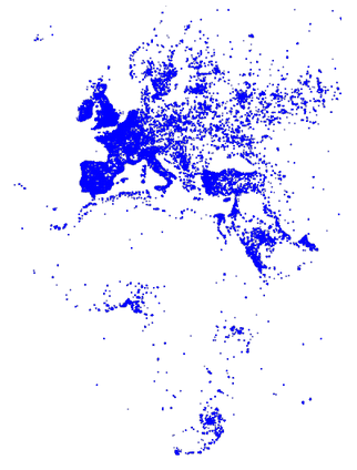
See the Vega at a Glance source code used in this example.

When you are ready to create your own Vega visualizations, look at the Tutorials and Reference documents to learn more.

Defining the Source Data¶

The Vega JSON structure maps data to geometric primitives.

A first task is to specify the data source. You can either define data statically or use a SQL query. This examples uses a SQL query to get tweet geolocation information from a tweets database:

SELECT goog_x as x, goog_y as y, tweets_nov_feb.rowid FROM tweets_nov_feb

The resulting SQL columns can be referenced in other parts of the specification to drive visualization elements. In this example, the projected columns are goog_x and goog_y, which are renamed x and y, and rowid, which is a requirement for hit-testing.

Creating a Visualization using Vega¶

The Vega specification for this example includes the following top-level properties:

height and width, which define the height and width of the visualization area.
data, which defines the data source. The SQL data described above is defined here with the label tweets for later referencing.
marks, which describes the geometric primitives used to render the visualization.
scales, which are referenced by marks to map input domain values to appropriate output range values.

Here is the full Vega specification used in this example:

const exampleVega = {
  "width": 384,
  "height": 564,
  "data": [
    {
      "name": "tweets",
      "sql": "SELECT goog_x as x, goog_y as y, tweets_nov_feb.rowid FROM tweets_nov_feb"
    }
  ],
  "scales": [
    {
      "name": "x",
      "type": "linear",
      "domain": [
        -3650484.1235206556,
        7413325.514451755
      ],
      "range": "width"
    },
    {
      "name": "y",
      "type": "linear",
      "domain": [
        -5778161.9183506705,
        10471808.487466192
      ],
      "range": "height"
    }
  ],
  "marks": [
    {
      "type": "points",
      "from": {
        "data": "tweets"
      },
      "properties": {
        "x": {
          "scale": "x",
          "field": "x"
        },
        "y": {
          "scale": "y",
          "field": "y"
        },
        "fillColor": "blue",
        "size": {
          "value": 3
        }
      }
    }
  ]
};

The following sections describe the top-level Vega specification properties.

Define the Visualization Area Dimensions¶

The width and height properties define a visualization area 384 pixels wide and 564 pixels high:

"width": 384
"height": 564

The scales position encoding properties map the marks into this visualization area.

Define the Marks¶

The marks property defines visualization geometric primitives. The MapD Vega implementation defines the following primitive types:

points A point
polys A polygon
symbol A geometric symbol, such as a circle or square

Each primitive type has a set of properties that describe how the primitive is positioned and styled.

This example uses points to represent the tweets data:

"marks": [
  {
    "type": "points",
    "from": {
      "data": "tweets"
    },
    "properties": {
      "x": {
        "scale": "x",
        "field": "x"
      },
      "y": {
        "scale": "y",
        "field": "y"
      },
      "fillColor": "blue",
      "size": {
        "value": 3
      }
    }
  }
]

Points support the following properties:

x The x position of the point in pixels.
y The y position of the point in pixels.
size The diameter of the point in pixels.
fillColor The color of the point.

The points in the example reference the tweets SQL data and use the x and y columns from the SQL to drive the position of the points. The positions are appropriately mapped to the visualization area using scales as described in Scale Input Domain to Output Range. The fill color is set to blue and point size is set to three pixels.

Scale Input Domain to Output Range¶

The scales definition maps data domain values to visual range values, where the domain property determines the input domain for the scale. See the d3-scale reference for background information about how scaling works.

This example uses linear scales to map mercator-projected coordinates into pixel coordinates for rendering.

"scales": [
  {
    "name": "x",
    "type": "linear",
    "domain": [
      -3650484.1235206556,
      7413325.514451755
    ],
    "range": "width"
  },
  {
    "name": "y",
    "type": "linear",
    "domain": [
      -5778161.9183506705,
      10471808.487466192
    ],
    "range": "height"
  },
]

The x and y scales use linear interpolation to map point x- and y-coordinates to the width and height of the viewing area. The width and height properties are predefined keywords that equate to the range [0, <current width>] and [0, <current height>].

After completing the Vega specification, you send the JSON structure to the backend for rendering.

Connecting to the Server and Rendering the Visualization¶

The following steps summarize the rendering and visualization sequence:

Instantiate the MapdCon object for connecting to the backend.
Call the connect method with server information, user credentials, and data table name.
Provide the renderVega() callback function to connect() and include the Vega specification as a parameter.
Display the returned PNG image in you client browser window.

MapD uses Apache Thrift for cross-language client communication with the backend. Include the following JavaScript Thrift interface libraries and the mapd-connector, which includes the renderVega() function:

<script src="js/thrift.js"></script>
<script src="js/mapd.thrift.js"></script>
<script src="js/mapd_types.js"></script>
<script src="js/mapd-connector.js"></script>

The following example encapsulates the connect, render request, and response handling sequence:

var conn = new MapdCon()
  .protocol("http")
  .host("myserver.mapd.com")
  .port("9092")
  .dbName("testdb")
  .user("testuser")
  .password("mypassword")
  .connect(function(error, con) {
    var results = con.renderVega(1, JSON.stringify(exampleVega));
    var blobUrl = 'data:image/png;base64,' + results.image;
    var w=window.open('about:blank','backend-rendered png');
    w.document.write("<img src='"+blobUrl+"' alt='backend-rendered png'/>")
  });

Next Steps¶

This example demonstrated the basic concepts for understanding and using Vega. To become comfortable with Vega, try this example using your own MapD instance, changing the MapdCon() parameters according to match your host environment and database.

As you gain experience with Vega and begin writing your own applications, you can find the information you need to take full advantage of Vega in the Reference document. Use the Tutorials document as a resource of common Vega usage examples, beginning with Tutorials Getting Started. All of the source code for this example and the tutorials can be found in Example Source Code.